One core idea of emulation is to represent the ensemble of outputs of a complicated simulator in a reduced basis. The battle-horse algorithm to do this is the famous PCA, a.k.a POD, a.k.a SVD, a.k.a EOF, a.k.a. EBD, a.k.a. KLD, a.k.a. …
Really, this algorithm has a different name in each community that uses it! I did not invest much time in finding whether this is due to simultaneous discoveries, or due to researchers not looking into other communities to see what already exist (i.e. re-inventing the wheel and calling it differently), or due to mischievous re-naming to get published. In case of the first there is nothing to do but wait (and hope) for unification. The second is something shouldn’t be common anymore, specially in the age of the internet. The third and last is unforgivable, it is more common than what I would like to accept, and is caused by the stupid pressure to publish a lot (instead of good stuff). I believe that the true cause is a mix of all three.
Anyways, I hope new researchers, with young blood, are more careful, ethical, and worry less about piling up disposable articles.
As I said at the beginning, one very useful approach to accelerate a complicated simulator is to try to represent the ensemble of outputs in a reduced basis. Generally this is something of the form
$$ \mathbf{y}(t,\mathbf{\lambda}) = \sum_{i=1}^N \mathbf{c}_i(\mathbf{\lambda}) \varphi_i(t) $$
where \(\mathbf{y}(t,\mathbf{\lambda})\) is the output of the simulator, here assumed to depend on time and some parameter vector \(\mathbf{\lambda}\). In the Ansatz above, we try to put the time dependence in some parameter independent basis \(\varphi_i(t)\), which is hopefully small. The dependence on the parameters is present only in the coefficients of the basis. Put in words, we try to represent any output of the simulator as a linear combination of a fixed basis. In this representation, we need to learn only the parameter dependence of the basis coefficients. We learn this dependence from outputs of the simulator obtained with different parameters, i.e.e the training data. When the basis is small this can provide a boost in the calculation time of outputs at new parameter values. The size of the basis is related to the complexity of the signals the simulator generates, more complex outputs require more basis elements to generate a good representation.
SVD decomposition
A very efficient way of obtaining the basis \(\varphi_i(t)\) is by applying the Singular Value Decomposition (SVD) to the so called snapshots matrix (or data matrix) \(\mathbb{Y}\) which contains the recorded simulation outputs in its columns
$$ \mathbb{Y} = \begin{bmatrix} y(t,\mathbf{\lambda}_1) & \ldots & y(t,\mathbf{\lambda}_n)\end{bmatrix} $$
This way of obtaining the basis is equivalent to:
-
Principal Components Analysis (PCA): well know in machine learning and statistics and used for dimensionality reduction.
-
Proper Orthogonal Decomposition (POD): popular in structural mechanics, physics, and theory of differential equations.
-
Karhunen-Loève Decomposition (KLD): also well known in statistics.
-
Empirical Orthogonal Functions (EOF): popular among wind and solar power researchers.
-
…
The list is really long and it gets longer the more I read from different research fields.
Of course there are other decomposition algorithms that are not equivalent to SVD. For example there is Nonnegative Matrix Factorization (NMF), Independent Component Analysis, Anechoic Mixing Models, my own work on kinematic chains using the Dynamic Decomposition Method1, and the many decompositions used in Compressed Sensing. All these other methods are also valid approaches for emulation. They can be particularly useful if we have prior information about the basis, or if we want the basis to have a given property for the sake of interpretability of the decomposition (this is seldom required in emulation since the objective is just to accelerate the simulator and not much more).
A very simple example is implemented in the script s_svd_ode.m, where the motion of the pendulum is reduced to an interpolation problem. The parameter vector contains the initial angle of the pendulum and the initial speed. In this example only 4 basis elements are needed to emulate the pendulum with an error of about 1%. you can see the surfaces of these coefficients in the plots below
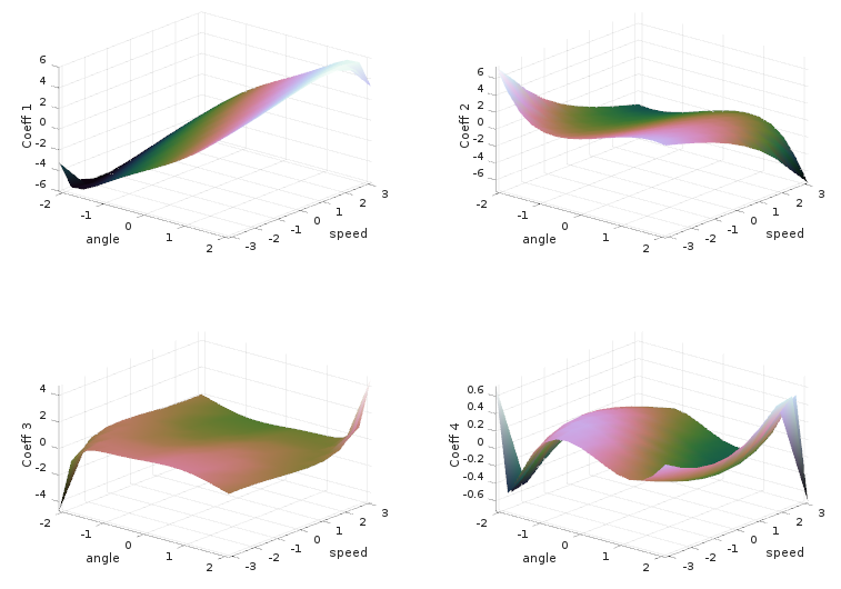
The 4 basis coefficients as function of the initial angle and velocity of the pendulum. Interpolation is used to emulate parameters not present in the training data.
We presented a concrete example of application of SVD and MNF in our publication2, under the name Data-driven emulation.
Similar ideas are applied in model order reduction (you can learn about the difference between emulation and MOR in this post), you can read about them in Reduced Basis Method for PDEs3 and in POD for dynamical systems 4.
Running the aglorithm
The file s_svd_ode.m contains a GNU Octave script. To run it, you will need Octave and the function pod.m. Put both file sin the same folder and call the script from the Octave prompt.
References
-
Carbajal, J. P. (2012). Harnessing Nonlinearities: Generating Behavior from Natural Dynamics. University of Zürich. https://doi.org/10.5167/uzh-66463 ↩︎
-
Carbajal, J. P., Leitão, J. P., Albert, C., & Rieckermann, J. (2017). Appraisal of data-driven and mechanistic emulators of nonlinear simulators: The case of hydrodynamic urban drainage models. Environmental Modelling & Software, 92, 17–27. http://doi.org/10.1016/j.envsoft.2017.02.006. Arxiv: https://arxiv.org/abs/1609.08395 ↩︎
-
Quarteroni, A., Manzoni, A., & Negri, F. (2015). Reduced Basis Methods for Partial Differential Equations: An Introduction. Springer International Publishing. ↩︎
-
Volkwein, S. (2013). Proper orthogonal decomposition: Theory and reduced-order modelling. Lecture Notes, University of Konstanz. http://www.math.uni-konstanz.de/numerik/personen/volkwein/teaching/POD-Book.pdf ↩︎