So you have your nifty numerical simulator that captures all the details of the complex device you want to model, everything! You got your digital twin, and for a while everything is OK.

There comes the day in which you want to use your simulator in ways that go beyond the constraints imposed by the physical world … well, isn’t that the reason why we build simulators?

You want to:

1. optimize the design of your device
2. find out the values of parameters of your device that are hard or impossible to measure (i.e. system identification)
3. use the model to predict the behavior of your device under different situations and control it in realtime.

At this point you realize that your nifty model is just too slow. Maybe a single simulation is many times faster than reality, lets say a simulation of your device running for months takes a few minutes, but applications 1.-3. require thousands of simulations, and even a runtime of a few minutes make those applications impractical.

So, what do you do? First, do not panic, you are not alone. This problem is quite common and there is a whole field of applied science that deals with it. In a nutshell: you need to speed-up your model by making it specific to the problem at hand.

Problem specification

To speed-up your simulator you need to check a few properties of the usage you have planned for it. In particular you want to check if you actually need all the details that your simulator provides. For example, a simulator based on the Finite Element Method (FEM) will produce a huge amount of values that you might not need to actually get the information you need for your application.

Loosely speaking, numerical simulators used in applications like the ones enumerated in the previous section have a fan-out/fain-in structure. Let an image explain this idea:

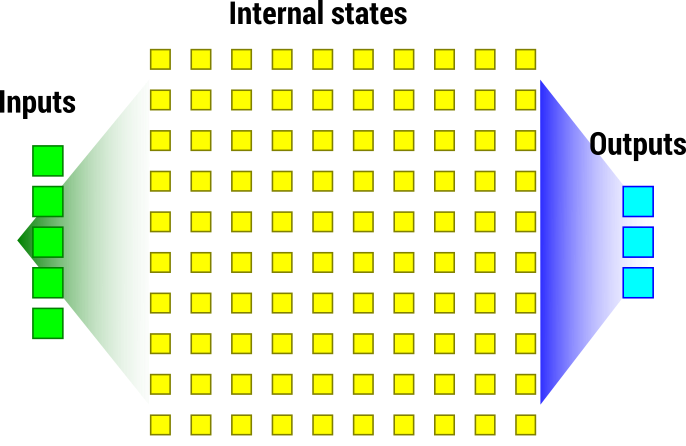
The fan-out part comes from the way inputs, e.g. boundary conditions, actuations, parameter values, etc., are mapped to internal states of the simulator (usually many … many!). Continuing with the FEM example, a few parameters defining the problem will produce hundreds or thousands of nodal values. Your simulator spends precious time keeping track of this plethora of values.

The fan-in part is given by the application at hand. Usually the application does not need the whole set of internal states, e.g. you might be interested in the signal produced by a sensor obtained from the average of states over a small region of your domain. In such (pervasive!) situations the quantity of output values is much smaller than the dimension (order) of the internal states of the simulator. Your simulator, by the way, is establishing a relation between the inputs and the outputs of your problem.

The natural question is then: can we find a smaller model that establishes the same (or a similar) relation between inputs and outputs? And the answer is generally yes, such reduced model exists.

Reduced models

The general way of reducing a model, and well suited for models based on differential equations (we will mainly refer to these), is via Model Order Reduction (MOR). MOR methodologies use information from your simulator and a set of simulations (snapshots) to create a reduced model that behaves very much like your detailed simulator.

MOR methodologies based on projections build a model with a structure derived from the structure of your simulator and with parameters adapted to reproduce the outputs of your simulator:

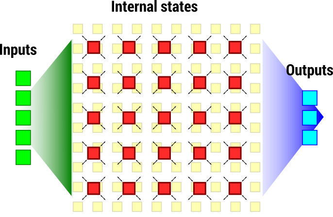
These methodologies give you some information about the internal states of the detailed simulator, but “blurred out”. It is like looking at a picture with your eyes ajar: you still see the picture, but textures and patterns with small details are blurred out (for the physicist out there: it is a kind of coarse-graining). The reduced model, having much fewer states and capturing the most important aspects of the input-output relation, spends less time in internal calculations and offers a speed-up.

Ey! Why not we take this to the extreme and get rid of all internal states? Enter emulation…

Emulators

Emulation takes MOR to its natural limit and uses only snapshots of your simulations to learn the input-output relation.

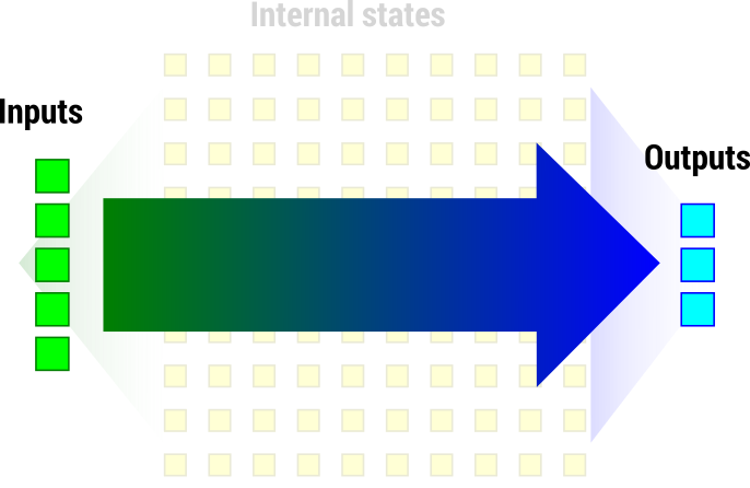
Emulation is a regression problem, even more, it is an interpolation and falls within the realm of Machine Learning and Scattered Data Approximation¹. Emulation will give you the highest speed-up attainable, but it is not always feasible.

If emulation exploits information from your simulator it is called mechanistic or invasive, and if it does not then is called data-driven (see this article² for a discussion). Having information about the simulator that generated the snapshots helps guessing the input-output relation far away from the given data.

Data-driven emulation is simpler to apply than mechanistic emulation and MOR. That is why you should try it first of all.

Recap

MOR and emulation, the extreme case, can help you with your speed problem. But there is no free lunch: to create any of these faster models, you will still need to run some simulations and then apply methods for the creation of the effective model.

Data-driven emulation uses no information about your simulator (besides the data), therefore the error of its predictions for inputs far away from the data is uncontrollable. Mechanistic emulation migth produce better trends outside the data scope, since it uses some information about the simulator structure. This is also the case with MOR.

An important difference between MOR and Emulation is that the former allows you to represent the (blurred) internal states of your simulator, while the latter does not.

References